
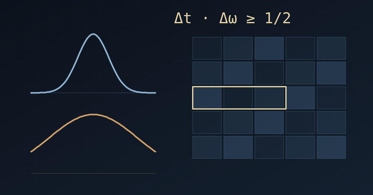
The ordinary Fourier transform is a unitary transform: information is fully preserved, and the inverse transform reconstructs the original signal exactly. This commonly raises a question: if not a single bit of information is lost, why does “uncertainty” still exist? The conclusion of this article is that the uncertainty principle constrains not the total amount of information, but the local readability of that information. It should be stressed that unitarity belongs only to the ordinary Fourier transform: its windowed version (the short-time Fourier transform) and the wavelet transform are merely isometries, not unitary operators. They preserve the norm but are not surjective, and the reproducing-kernel structure of their range provides precisely the sharpest formulation of the uncertainty principle in the time-frequency domain. The article first states the Heisenberg–Weyl inequality and its proof, then explains through three mechanisms (the phase slope, the time-order invariance of the magnitude spectrum, and the reproducing kernel of the range) why invertibility does not provide local readability, and finally verifies the limits of the wavelet transform’s advantage with a cross-band dual-task example, from which a directly computable criterion for method selection is derived.
1. Problem Statement: Invertibility versus Readability
Two propositions at different levels must be distinguished (all of the following concern the ordinary Fourier transform; the windowed case is treated in Section 4.3):
| Proposition | Holds? | Level |
|---|---|---|
| The Fourier transform is invertible and no information is lost | Holds | Invertibility |
| $f(t)$ can be reconstructed exactly from $\hat f$, so the state at any instant is known | Holds | Invertibility |
| $\hat f(\omega)$ can be computed exactly from $f(t)$, so the frequency content is known | Holds | Invertibility |
| A joint density $P(t,f)$ exists from which “the frequency at time $t$” can be read | Does not hold | Readability |
| The instant can be localised to arbitrary precision and the frequency resolved to arbitrary precision simultaneously | Does not hold | Readability |
The first three rows belong to the domain of invertibility and the last two to the domain of readability; the two do not conflict. A common reasoning error is to conjoin rows 2 and 3 and erroneously infer row 4. $f(t)$ and $\hat f(\omega)$ are two mutually exclusive representations of the same information and cannot both be presented at high resolution on the same chart.
2. The Heisenberg–Weyl Inequality
2.1 Statement of the Theorem
Let $f \in L^2(\mathbb{R})$, $\lVert f \rVert_2 = 1$, with Fourier transform $\hat f(\omega)$. Define the centres and spreads in time and frequency:
$$ t_0 = \int t \lvert f(t)\rvert^2 dt, \qquad \Delta t^2 = \int (t-t_0)^2 \lvert f(t)\rvert^2 dt $$
$$ \omega_0 = \frac{1}{2\pi}\int \omega \lvert \hat f(\omega)\rvert^2 d\omega, \qquad \Delta\omega^2 = \frac{1}{2\pi}\int (\omega-\omega_0)^2 \lvert \hat f(\omega)\rvert^2 d\omega $$
Then it always holds that
$$ \Delta t \cdot \Delta \omega \geq \frac{1}{2} \qquad\Longleftrightarrow\qquad \Delta t \cdot \Delta f \geq \frac{1}{4\pi} \approx 0.0796 $$
In signal analysis this relation is called the Gabor limit. It is the same mathematical theorem as the position–momentum uncertainty relation in quantum mechanics, with only the pair of conjugate variables replaced.
2.2 Proof
Without loss of generality take $t_0 = \omega_0 = 0$. By Parseval’s theorem and $\mathcal{F}[f^{\prime}] (\omega) = i\omega\hat f(\omega)$, one has $\Delta\omega^2 = \lVert f^{\prime} \rVert^2$. Hence
$$ \Delta t^2 \Delta\omega^2 = \lVert tf \rVert^2 \lVert f^{\prime} \rVert^2 \geq \lvert \langle tf, f^{\prime} \rangle \rvert^2 \geq \lvert \operatorname{Re}\langle tf, f^{\prime} \rangle \rvert^2 $$
The first inequality is the Cauchy–Schwarz inequality. Noting that $2\operatorname{Re}\big(\overline{f}f^{\prime}\big) = (\lvert f\rvert^2)^{\prime}$, integration by parts of the real-part term gives:
$$ \operatorname{Re}\langle tf, f^{\prime} \rangle = \frac{1}{2}\int t \big(\lvert f\rvert^2\big)^{\prime} dt = -\frac{1}{2}\int \lvert f\rvert^2 dt = -\frac{1}{2} $$
Substituting back yields $\Delta t^2 \Delta\omega^2 \geq 1/4$, which completes the proof.
2.3 Condition for Equality
Equality in Cauchy–Schwarz requires $f^{\prime} = -\lambda t f$ ($\lambda > 0$), whose solution is
$$ f(t) = C e^{-\lambda t^2/2} $$
That is, the lower bound is attained if and only if $f$ is a Gaussian (or a modulated and translated Gaussian). Taking $f(t) = (\pi\sigma^2)^{-1/4}e^{-t^2/2\sigma^2}$, one has $\hat f(\omega) \propto e^{-\sigma^2\omega^2/2}$, and it can be verified directly that:
- the variance of $\lvert f \rvert^2$ is $\sigma^2/2$, so $\Delta t = \sigma/\sqrt2$
- the variance of $\lvert \hat f \rvert^2$ is $1/(2\sigma^2)$, so $\Delta\omega = 1/(\sigma\sqrt2)$
- the product is exactly $1/2$
The parameter $\sigma$ can only transfer uncertainty between time and frequency; it cannot reduce the total. This is the theoretical basis for the choice of a Gaussian window in the Gabor transform.
2.4 Limiting Cases and Corollaries
| Signal | $\Delta t$ | $\Delta\omega$ |
|---|---|---|
| $\delta(t-t_0)$ | $0$ | $\infty$ |
| $e^{i\omega_0 t}$ | $\infty$ | $0$ |
| Gaussian $e^{-t^2/2\sigma^2}$ | $\sigma/\sqrt2$ | $1/(\sigma\sqrt2)$ |
The Paley–Wiener theorem further implies that no nonzero function is compactly supported in both the time domain and the frequency domain. This explains why finite-length filters necessarily possess a transition band.
3. Tiling of the Time-Frequency Plane
The geometric interpretation of the above constraint is that the area of each “resolution cell” in the time-frequency plane has a lower bound; different transforms merely tile the same plane with cells of different shapes.
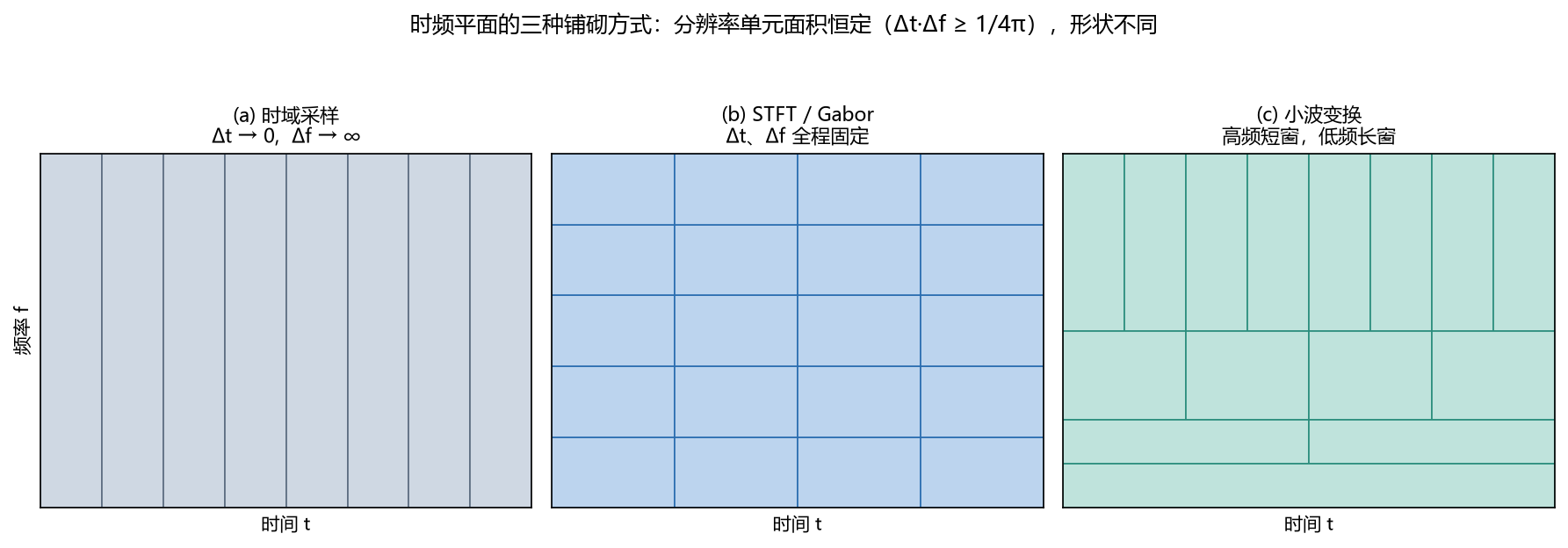
- Time-domain sampling: the cell degenerates into a vertical strip spanning the full band, $\Delta t \to 0$, $\Delta f \to \infty$
- STFT / Gabor: the cell is a rectangle of fixed shape, with the same window length shared across the full band
- Wavelet transform: the cell shape dilates and contracts with scale. At scale $a$ the wavelet atom is $a^{-1/2}\psi\left(\frac{t-b}{a}\right)$; its time spread is proportional to $a$ and its frequency spread inversely proportional to $a$, so the product is independent of $a$
The cell areas of all three are subject to the same constraint $\Delta t\cdot\Delta f \geq 1/(4\pi)$. Wavelets do not break this constraint; they only redistribute resolution according to frequency. The precise origin of this lower bound in windowed analysis is the reproducing kernel of the transform’s range, i.e. the ambiguity function of the analysis window itself; see Section 4.3 for details.
4. Why Invertibility Does Not Provide Local Readability
4.1 Mechanism 1: Time Information Is Encoded in the Phase Slope
Consider the most extreme time-localised event, an instantaneous impulse $\delta(t-t_0)$, whose Fourier transform is
$$ \mathcal{F}[\delta(t-t_0)] (\omega) = e^{-i\omega t_0} $$
The magnitude spectrum is identically 1 and completely flat along the entire frequency axis. The information “the event occurs at $t_0$” is not lost at all, but it does not reside in any single frequency component; it exists in the form of the slope of the phase with respect to frequency:
$$ \frac{d\varphi}{d\omega} = -t_0 $$
Measuring the slope of a straight line requires a sufficiently long baseline in the independent variable. If the observation bandwidth is only $B$, then
$$ \delta t_0 \sim \frac{1}{B} $$
This is another face of the uncertainty principle: the time-localisation precision is determined by the span of observation in the frequency domain.
4.2 Mechanism 2: The Magnitude Spectrum Cannot Distinguish Temporal Order
Construct a pair of contrasting signals: $A(t)$ is a modulated signal that is low-frequency first and high-frequency afterwards, and $B(t) = A(t_{\rm end} - t)$ is its time reversal. By the time-reversal property of the Fourier transform, for real signals
$$ \hat B(\omega) = \overline{\hat A(\omega)} e^{-i\omega t_{\rm end}} \qquad\Longrightarrow\qquad \lvert \hat B(\omega) \rvert \equiv \lvert \hat A(\omega) \rvert $$
The magnitude spectra of the two are exactly equal point by point. However finely the frequency axis is subdivided, the magnitude spectrum cannot determine the order of events; the difference resides 100% in the phase. The inverse transform can of course distinguish the two perfectly, but this requires a global reconstruction using the complete phase over the full band at full precision; “reading off the instant at a glance from the spectrum” is a local read-out and is precisely the forbidden operation.
4.3 Mechanism 3: The Range of Windowed Analysis Is Constrained by a Reproducing Kernel
The preceding two subsections concern the ordinary Fourier transform. On passing to windowed analysis the operator properties change, and this change yields the sharpest formulation of the uncertainty principle in the time-frequency domain.
Let the window $g$ satisfy $\lVert g\rVert_2 = 1$. The short-time Fourier transform (with the $e^{-2\pi i t\omega}$ convention) is
$$ V_g f(b, \omega) = \int f(t) \overline{g(t-b)} e^{-2\pi i t\omega} dt $$
From the Moyal orthogonality relation
$$ \langle V_{g_1} f_1, V_{g_2} f_2\rangle_{L^2(\mathbb{R}^2)} = \langle f_1, f_2\rangle \overline{\langle g_1, g_2\rangle} $$
taking $g_1 = g_2 = g$ and $f_1 = f_2 = f$ gives $\lVert V_g f\rVert_{L^2(\mathbb{R}^2)} = \lVert f\rVert_{L^2(\mathbb{R})}$, so $V_g$ preserves the norm. However, $V_g$ maps functions of one variable to functions of two variables, so its range must be a proper closed subspace of $L^2(\mathbb{R}^2)$, and it cannot be surjective. Hence
$$ V_g^{\ast}V_g = I, \qquad V_g V_g^{\ast} = P \neq I $$
where $P$ is the orthogonal projection onto the range. $V_g$ is an isometry, not a unitary operator; unitarity requires a bijective isometry. The same holds for the continuous wavelet transform $W_\psi$.
| Transform | Norm-preserving | Surjective | Unitary |
|---|---|---|---|
| Fourier transform $\mathcal{F}$ | Yes | Yes | Yes |
| Short-time Fourier transform $V_g$ | Yes | No | No |
| Continuous wavelet transform $W_\psi$ | Yes | No | No |
Reproducing kernel of the range. The range is a reproducing kernel Hilbert space: every admissible time-frequency map $F = V_g f$ must satisfy the fixed-point equation
$$ F(z) = \int_{\mathbb{R}^2} F(z^{\prime}) \langle \pi(z^{\prime})g, \pi(z)g\rangle dz^{\prime} $$
where $\pi(z)$ is the time-frequency shift operator, and the modulus of the kernel $\lvert\langle \pi(z^{\prime})g, \pi(z)g\rangle\rvert = \lvert V_g g(z-z^{\prime})\rvert$ is exactly the ambiguity function of the window itself. This yields the precise formulation of the uncertainty principle in the STFT domain:
Every time-frequency map is a fixed point of convolution with the ambiguity function of the window, so its concentration cannot be finer than the time-frequency footprint of the window itself.
For a Gaussian window, the area of this footprint equals exactly the lower bound $1/(4\pi)$. The impossibility of drawing an arbitrarily sharp time-frequency map is not a deficiency of algorithms; a sharp map simply does not lie in the range.
Numerical verification. For a fully dense discrete Gabor system with $N = 64$, a Gaussian window and a hop of 1 ($V$ maps an $N$-dimensional vector to an $N\times N$ matrix), the results are as follows (code in Appendix A.1):
| Test | Result | Meaning |
|---|---|---|
| $\lVert Vf\rVert^2/\lVert f\rVert^2$ | Constant $64 = N\lVert g\rVert^2$, independent of $f$ | Norm-preserving (isometry) |
| $\lVert V^{\ast}Vf/N - f\rVert/\lVert f\rVert$ | $4.8\times10^{-15}$ | A left inverse exists; exact reconstruction is possible |
| Random $R$, $\lVert PR-R\rVert/\lVert R\rVert$ | $0.991$ | $R$ lies almost entirely outside the range |
| $\lVert P(PR)-PR\rVert/\lVert PR\rVert$ | $5.6\times10^{-15}$ | $P$ is idempotent and is indeed a projection |
| Admissible time-frequency map $F$: $\lVert PF-F\rVert/\lVert F\rVert$ | $4.8\times10^{-15}$ | The reproducing-kernel property holds |
| Dimension of range / dimension of ambient space | $64/4096 = 1.56%$ | The range is a very thin subspace |
That is: more than 98% of the functions on the time-frequency plane are not the short-time Fourier transform of any signal.
After discretisation the STFT constitutes a Gabor frame, which is generally redundant; at critical density, the Balian–Low theorem (Reference 7) further shows that good time-frequency localisation and a Riesz basis cannot be obtained simultaneously.
4.4 An Intuitive Analogy
Suppose the traffic light at an intersection has a constant period of 60 s. After 1 h of continuous recording, an FFT shows a spectral line at $1/60 = 16.67\ \mathrm{mHz}$, and the inverse transform recovers the red/green state at any instant exactly. Here “both time and frequency are known” holds, not because the Fourier transform circumvents the uncertainty principle, but because the signal is stationary: the frequency does not change over time, so the problem of joint localisation is never posed.
Now consider an adaptive traffic light that switches at some instant from a 60 s period to a 40 s period, and pose the joint question: “What is the period, and when does it change?” Distinguishing the two periods requires a frequency resolution finer than
$$ \Delta f = \frac{1}{40} - \frac{1}{60} = 8.33\ \mathrm{mHz} $$
Even with an optimal Gaussian window, the theoretical lower bound $\Delta t \geq 1/(4\pi\Delta f)$ gives $\Delta t \geq 9.55\ \mathrm{s}$. The statement “the period changes from 60 s to 40 s, and the switch occurs within ±1 s of a certain instant” cannot hold simultaneously in mathematical terms, regardless of sampling rate, data volume or algorithmic sophistication.
5. Numerical Example: A Cross-Band Dual Task
5.1 Distinguishing Two Kinds of Constraint
Before discussing whether wavelets hold an advantage, two constraints of entirely different nature must be distinguished:
| Constraint | Content | Removable? |
|---|---|---|
| Physical constraint | A single analysis atom must satisfy $\Delta t\cdot\Delta f \geq 1/(4\pi)$; its precise form in the time-frequency domain is the reproducing-kernel constraint of Section 4.3 | Not removable |
| Artificial constraint | The STFT shares the same window across the full band, i.e. all atoms have the same shape | Removable |
This yields the key to deciding whether wavelets can hold an advantage:
- When the two tasks lie in the same frequency band, they compete for the same resolution cell and must be served by the same atom, which runs into the physical constraint. The compatibility condition is then $\Delta t_{\rm sep}\cdot\Delta f_{\rm sep} \gtrsim 1/\pi$; if it is not satisfied, no method (including wavelets) has a solution.
- When the two tasks lie in two widely separated frequency bands, they are served by atoms of different scales, each of which only needs to satisfy the physical constraint individually, and the atoms do not compete. The failure of the STFT then stems purely from the artificial constraint, which wavelets remove by using different atoms for different frequencies.
The example constructed in this section belongs to the latter case.
5.2 Signal Design
A rotating-machinery fault-diagnosis scenario is adopted ($f_s = 10\ \mathrm{kHz}$, duration 2 s):
- Low-frequency task: the fundamental frequencies of two shafts, 24.0 Hz and 30.0 Hz ($\Delta f_{\rm sep} = 6\ \mathrm{Hz}$). Question: which shaft is unbalanced
- High-frequency task: 3000 Hz resonance impacts excited by a bearing defect, occurring at $t = 1.000\ \mathrm{s}$ and $t = 1.015\ \mathrm{s}$ ($\Delta t_{\rm sep} = 15\ \mathrm{ms}$). Question: when do the impacts occur
The two questions have the same form (“which one” and “when”), but their requirements on the analysis parameters point in opposite directions, and they lie in two frequency bands separated by a factor of 111.
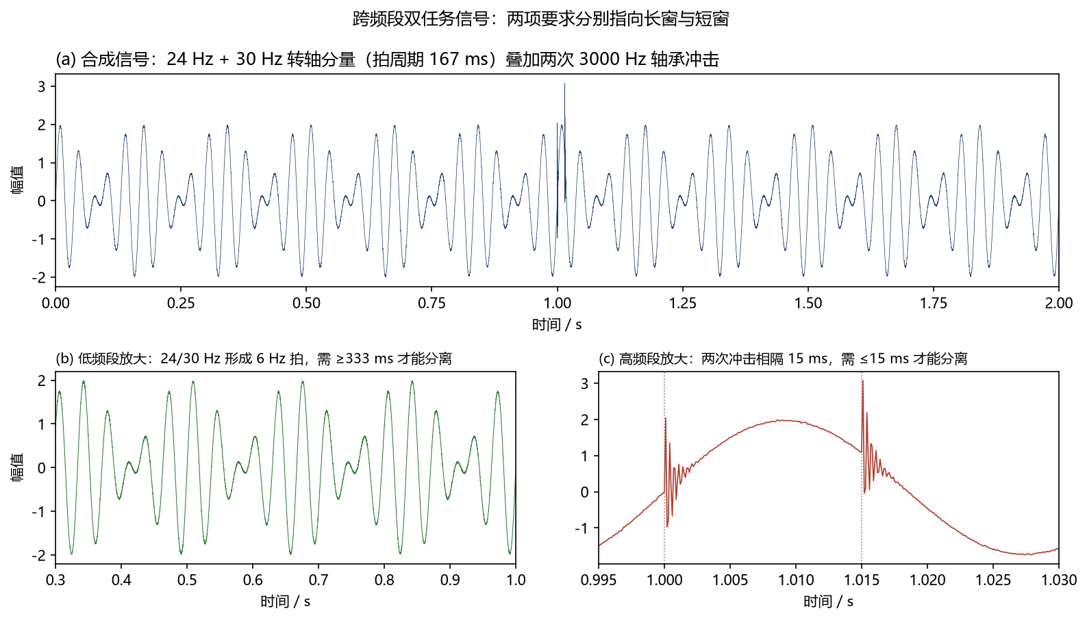
The product $\Delta t_{\rm sep}\cdot\Delta f_{\rm sep} = 0.015 \times 6 = 0.090$ is below the single-atom dual-task threshold $1/\pi = 0.318$, so no STFT with a single window length has a solution; however, it exceeds the absolute lower bound $1/(4\pi) = 0.0796$, and the two tasks lie at different frequencies, so the problem is not forbidden by the physical constraint.
5.3 Analytical Feasible Region
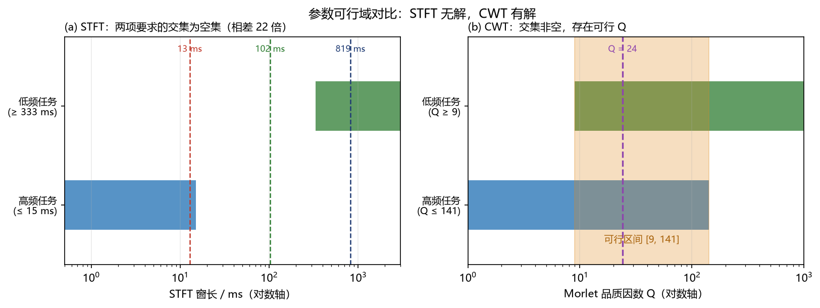
The STFT must satisfy both requirements with a single window length. Using the Hann-window main-lobe width $2/T_{\rm win}$ as the resolution criterion:
$$ T_{\rm win} \geq \frac{2}{\Delta f_{\rm sep}} = 333\ \mathrm{ms} \quad\wedge\quad T_{\rm win} \leq \Delta t_{\rm sep} = 15\ \mathrm{ms} \quad\Longrightarrow\quad \text{feasible region} = \varnothing $$
The lower limit is 22 times the upper limit.
The free parameter of the CWT is the quality factor $Q$ ($Q = \omega_0$ for the Morlet wavelet). Under the amplitude convention, its resolution scales with frequency:
$$ \Delta f = \frac{f}{Q}, \qquad \sigma_t = \frac{Q}{2\pi f}, \qquad \sigma_t \cdot \Delta f = \frac{1}{2\pi}\ \text{(independent of frequency)} $$
The two requirements are imposed at their respective frequencies and therefore do not conflict:
$$ Q \geq \frac{2 f_L}{\Delta f_{\rm sep}} = \frac{2\times 27}{6} = 9.0 \quad\wedge\quad Q \leq \pi f_H \Delta t_{\rm sep} = \pi\times 3000\times 0.015 = 141 $$
$$ \Longrightarrow\quad \text{feasible region} = [9,\ 141] \neq \varnothing $$
With $Q = 24$, the actual resolutions are: at 27 Hz, $\Delta f = 1.12\ \mathrm{Hz} \ll 6\ \mathrm{Hz}$; at 3000 Hz, $\sigma_t = 1.27\ \mathrm{ms} \ll 15\ \mathrm{ms}$. Both requirements are met with ample margin.
5.4 Numerical Results
For each method a single full-band time-frequency map is given (logarithmic frequency axis, 180 ms time window), so that both tasks can be read simultaneously on the same map: cyan dashed lines mark 24 and 30 Hz, and green dashed lines mark 1.000 and 1.015 s.
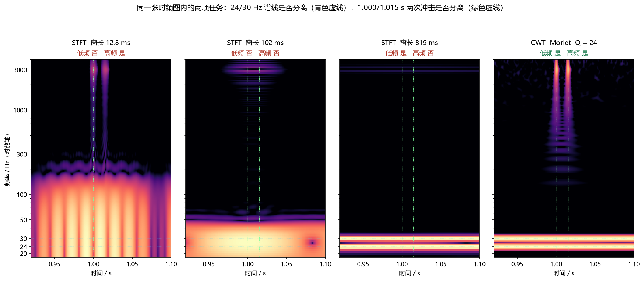
| Method | Resolves 24/30 Hz | Resolves 1.000/1.015 s | Dual task |
|---|---|---|---|
| STFT 12.8 ms | No | Yes | Fail |
| STFT 102 ms | No | No | Fail |
| STFT 819 ms | Yes | No | Fail |
| CWT $Q=24$ | Yes | Yes | Pass |
The criterion is the Rayleigh dip-depth criterion: two main peaks are judged resolved only if the valley between them is below 0.7 times the peak value. This criterion excludes spurious double peaks caused by amplitude ripple.
Only the CWT column exhibits both features simultaneously: at the low-frequency end, two distinct spectral lines lie at 24 and 30 Hz, and at the high-frequency end, two distinct vertical lines lie at 1.000 and 1.015 s. Each of the three STFT window lengths fails in at least one task, and the direction of failure shifts monotonically with window length: the short window preserves time, the long window preserves frequency, and the intermediate window preserves neither.
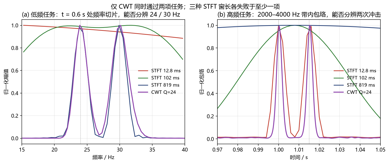
In the quantitative slices, the CWT curve is the only one that exhibits a double peak in both the left and right panels.
5.5 Image Details and Methodological Points
First, the diffuse band spanning the full width at 3000 Hz in the 819 ms panel. The impact energy is spread over 819 ms, far beyond the 180 ms display window, so it appears as a uniform horizontal band rather than vertical lines. The information is not lost; only the time localisation is completely smeared out.
Second, the fine horizontal fringes in the high-frequency region of the 102 ms and 819 ms panels. The fringe spacing is $1/\Delta t_{\rm sep} = 66.7\ \mathrm{Hz}$; these are interference fringes of the two impacts. A window longer than the impact interval records “two impacts” as “one event plus frequency-domain fringes”, which is another encoding of the same fact.
Third, both descriptions are correct. The 12.8 ms window gives the description “a single 27 Hz component whose amplitude beats at 6 Hz” (beat period 167 ms, clearly visible in the time-domain waveform); the 819 ms window gives the description “two independent components at 24 and 30 Hz”. Both describe the same signal and neither is wrong. The uncertainty principle does not destroy information; it only determines the form in which the information is presented. This is the same phenomenon as discussed in Section 4.
Fourth, zero-padding does not improve resolution. In the decision computation all three window lengths are zero-padded to 16384 points, giving a uniform frequency grid of $f_s/N_{\rm FFT} = 0.61\ \mathrm{Hz}$, far finer than the 6 Hz spacing. The frequency slice of the 12.8 ms window is smooth and adequately sampled, yet still shows only a single peak. Resolution is determined by the window length and is independent of the number of FFT points; zero-padding merely performs sinc interpolation of the spectrum and introduces no new information.
6. General Criterion: The Feasible-Region Width Ratio
Let the two tasks lie at frequencies $f_L$ (requiring frequency resolution $\Delta f_{\rm sep}$) and $f_H$ (requiring time resolution $\Delta t_{\rm sep}$), with $f_H > f_L$. From the two expressions of Section 5.3, define the feasible-region width ratio
$$ R = \frac{Q_{\max}}{Q_{\min}} = \frac{\pi}{2}\cdot\frac{f_H}{f_L}\cdot \Delta t_{\rm sep}\cdot\Delta f_{\rm sep} \approx 1.571\ \frac{f_H}{f_L}\ \Delta t_{\rm sep}\ \Delta f_{\rm sep} $$
The decision rule is:
- $R < 1$: wavelets have no solution
- $R \approx 1$: the feasible region degenerates and the solution is not robust
- $R \gg 1$: the feasible region is ample and wavelets hold a robust advantage
Equivalently, a wavelet solution requires
$$ \frac{f_H}{f_L} \geq \frac{2}{\pi}\cdot\frac{1}{\Delta t_{\rm sep}\cdot\Delta f_{\rm sep}} \approx \frac{0.637}{\Delta t_{\rm sep}\cdot\Delta f_{\rm sep}} $$
Substituting the example of this article: $\Delta t_{\rm sep}\cdot\Delta f_{\rm sep} = 0.090$ requires $f_H/f_L \geq 7.1$, whereas the actual value is 111, so $R = 15.7$ with ample margin. For comparison, if the two tasks both lie near 100 Hz ($f_H/f_L \approx 2.9$) with $\Delta t_{\rm sep}\cdot\Delta f_{\rm sep} = 0.16$, then $R = 0.74 < 1$ and wavelets likewise have no solution; this is exactly the case of “competing for the same resolution cell” described in Section 5.1.
The expression shows that the larger the frequency ratio of the two tasks and the looser their respective resolution requirements, the wider the feasible region of wavelets. $R$ can be computed directly from the task specifications before the analysis scheme is designed, without trial computation.
7. Conclusions and Scope of Application
The advantage of wavelets is not that they “break the uncertainty principle”, but that they “remove the artificial constraint of the STFT sharing a single window across the full band”. On this basis a clear method-selection criterion can be given:
- Wavelets should be used when the signal has a multiscale structure, the low-frequency components require high frequency resolution, the high-frequency components require high time resolution, and $R \gg 1$. Typical scenarios include rotating-machinery fault diagnosis, joint analysis of seismic first arrivals and surface waves, analysis of the ST segment and QRS complex in ECG signals, and transient electromagnetic responses.
- Wavelets are unnecessary when all objects of interest lie in the same frequency band (the constant-$Q$ property then offers no benefit, and a long-window STFT is preferable), or when the signal itself is stationary (a direct FFT suffices).
- Wavelets also have no solution when $R < 1$, i.e. the two tasks compete for the same resolution cell. In this case one must turn to nonlinear methods such as synchrosqueezing or reassigned spectrograms, or change the sensing modality, for example recording events directly with timestamps; event records undergo no time-frequency decomposition and are therefore not subject to this constraint.
Appendix: Reproducible Code
The environment is Python 3.14 + NumPy 2.4 + SciPy 1.18.
A.1 Verification of Operator Properties (Section 4.3)
# -*- coding: utf-8 -*-
"""The discrete STFT is an isometry but not a unitary operator"""
import numpy as np

rng = np.random.default_rng(7)
N = 64
k = np.arange(N)
E = np.exp(-2j * np.pi * np.outer(k, k) / N)          # E[m, t] = exp(-2i pi m t / N)
g = np.exp(-0.5 * ((k - N / 2) / (N / 8.0)) ** 2)
g = g / np.linalg.norm(g)                              # unit-norm Gaussian window
G = np.stack([np.roll(g, j) for j in range(N)], axis=1)   # G[t, n] = g[t-n]


def V(f):
    """Discrete STFT: N-dim vector -> N x N complex matrix (rows: frequency, columns: time shift)"""
    return E @ (f[:, None] * np.conj(G))


def Vstar(F):
    """Adjoint operator"""
    return np.einsum("mn,mt,tn->t", F, np.conj(E), G)


f1 = rng.standard_normal(N) + 1j * rng.standard_normal(N)
f2 = rng.standard_normal(N) + 1j * rng.standard_normal(N)
c = N * np.linalg.norm(g) ** 2

r1 = np.linalg.norm(V(f1)) ** 2 / np.linalg.norm(f1) ** 2
r2 = np.linalg.norm(V(f2)) ** 2 / np.linalg.norm(f2) ** 2
print("norm  : {:.10f}  {:.10f}   theory N||g||^2 = {:.10f}".format(r1, r2, c))
print("l-inv : ||V*Vf/c - f||/||f|| = {:.3e}".format(
    np.linalg.norm(Vstar(V(f1)) / c - f1) / np.linalg.norm(f1)))

R = rng.standard_normal((N, N)) + 1j * rng.standard_normal((N, N))   # arbitrary function on the time-frequency plane
PR = V(Vstar(R)) / c
print("onto  : ||PR - R||/||R||     = {:.4f}".format(
    np.linalg.norm(PR - R) / np.linalg.norm(R)))
print("idemp : ||P(PR) - PR||/||PR|| = {:.3e}".format(
    np.linalg.norm(V(Vstar(PR)) / c - PR) / np.linalg.norm(PR)))

F1 = V(f1)
print("kernel: ||PF - F||/||F||     = {:.3e}".format(
    np.linalg.norm(V(Vstar(F1)) / c - F1) / np.linalg.norm(F1)))
print("dim range {} / dim ambient space {} = {:.2f}%".format(N, N * N, 100.0 * N / N ** 2))
A.2 Cross-Band Dual-Task Decision (Section 5.4)
The following script reproduces the analytical feasible region and the decision table of the main text, excluding the plotting part.
# -*- coding: utf-8 -*-
"""Numerical decision for the cross-band dual task

Low-frequency task:  resolve the two shaft components at 24 / 30 Hz       -> requires a long window
High-frequency task: resolve two impacts 15 ms apart at 3000 Hz           -> requires a short window
Conclusion: every single STFT window length fails; the Morlet wavelet succeeds for Q in [9, 141].
"""
import numpy as np
from scipy.signal import ShortTimeFFT
from scipy.signal.windows import hann


def stft_mag(x, fs, N, hop, mfft):
    """Hann-window STFT magnitude. Zero-padded to mfft points so that the frequency grid is much finer than the resolution."""
    S = ShortTimeFFT(hann(N, sym=False), hop=hop, fs=fs, mfft=mfft, scale_to="magnitude")
    return np.abs(S.stft(x)), S.f, S.t(x.size)


def cwt_morlet(x, fs, freqs, Q):
    """Morlet continuous wavelet transform. Amplitude-preserving normalisation: a unit-amplitude sinusoid gives |W| = 1 at its own scale."""
    Xf = np.fft.fft(x)
    w = 2 * np.pi * np.fft.fftfreq(x.size, d=1 / fs)
    pos = w > 0
    out = np.empty((freqs.size, x.size))
    for i, fc in enumerate(freqs):
        a = Q / (2 * np.pi * fc)
        out[i] = np.abs(np.fft.ifft(Xf * (2.0 * np.exp(-(a * w - Q) ** 2 / 2) * pos)))
    return out


def resolved(y, thr=0.5, dip=0.7):
    """Rayleigh dip-depth criterion: two main peaks are judged resolved only if the valley between them is below dip times the peak value."""
    idx = [i for i in range(1, len(y) - 1)
           if y[i] > y[i - 1] and y[i] >= y[i + 1] and y[i] > thr]
    if len(idx) < 2:
        return False
    a, b = sorted(sorted(idx, key=lambda i: -y[i])[:2])
    return y[a:b + 1].min() <= dip * min(y[a], y[b])


def nrm(v):
    return v / v.max()


# ---------------------------------------------------------------- signal construction
fs = 10000.0
t = np.arange(0, 2.0, 1 / fs)
FL1, FL2, FH = 24.0, 30.0, 3000.0      # fundamental frequencies of the two shafts; bearing resonance frequency
TH1, TH2 = 1.000, 1.015                # instants of the two impacts
DF, DT = FL2 - FL1, TH2 - TH1          # 6 Hz; 15 ms
FL = 0.5 * (FL1 + FL2)

x = np.sin(2 * np.pi * FL1 * t) + np.sin(2 * np.pi * FL2 * t)
for t0 in (TH1, TH2):
    m = t >= t0
    x[m] += 2.5 * np.exp(-(t[m] - t0) / 6e-4) * np.sin(2 * np.pi * FH * (t[m] - t0))
x += 0.01 * np.random.default_rng(1).standard_normal(t.size)

# ---------------------------------------------------------------- analytical feasible region
T_LO = 2.0 / DF                 # STFT low-frequency task: Hann main lobe 2/T_win <= df_sep
T_HI = DT                       # STFT high-frequency task: T_win <= dt_sep
Q_MIN = 2 * FL / DF             # CWT low-frequency task: 2*Df = 2*f_L/Q <= df_sep
Q_MAX = np.pi * FH * DT         # CWT high-frequency task: 2*sigma_t = 2*Q/(2*pi*f_H) <= dt_sep
Q_USE = 24.0

print("ratio f_H/f_L = {:.0f},  dt_sep * df_sep = {:.3f}".format(FH / FL, DT * DF))
print("STFT: T_win >= {:.0f} ms and T_win <= {:.0f} ms  ->  empty set (factor {:.0f})"
      .format(T_LO * 1e3, T_HI * 1e3, T_LO / T_HI))
print("CWT : Q >= {:.1f} and Q <= {:.1f}  ->  [{:.0f}, {:.0f}], R = {:.1f}, use Q = {:.0f}"
      .format(Q_MIN, Q_MAX, Q_MIN, Q_MAX, Q_MAX / Q_MIN, Q_USE))
print("Q = {:.0f}: at {:.0f} Hz Df = {:.2f} Hz;  at {:.0f} Hz sigma_t = {:.2f} ms\n"
      .format(Q_USE, FL, FL / Q_USE, FH, Q_USE / (2 * np.pi * FH) * 1e3))

# ---------------------------------------------------------------- numerical decision
LO, HI = (15.0, 40.0), (2000.0, 4000.0)
rows = []
for N in (128, 1024, 8192):
    S, f, tt = stft_mag(x, fs, N, hop=20, mfft=16384)
    fm = (f >= LO[0]) & (f <= LO[1])
    r1 = resolved(nrm(S[fm, int(np.argmin(np.abs(tt - 0.60)))]))
    bm = (f >= HI[0]) & (f <= HI[1])
    env = nrm(np.sqrt((S[bm] ** 2).mean(axis=0)))
    tm = (tt >= 0.97) & (tt <= 1.05)
    rows.append(("STFT {:.0f} ms".format(N / fs * 1e3), r1, resolved(env[tm])))
    del S

freqs = np.geomspace(15.0, 4200.0, 340)
W = cwt_morlet(x, fs, freqs, Q=Q_USE)
lom = (freqs >= LO[0]) & (freqs <= LO[1])
him = (freqs >= HI[0]) & (freqs <= HI[1])
r1 = resolved(nrm(W[lom, int(np.argmin(np.abs(t - 0.60)))]))
env = nrm(np.sqrt((W[him] ** 2).mean(axis=0)))
tm = (t >= 0.97) & (t <= 1.05)
rows.append(("CWT Q={:.0f}".format(Q_USE), r1, resolved(env[tm])))

print("{:<14s}{:>10s}{:>10s}{:>9s}".format("method", "low-f", "high-f", "dual"))
print("-" * 46)
for name, r1, r2 in rows:
    print("{:<14s}{:>10s}{:>10s}{:>9s}".format(
        name, "resolved" if r1 else "merged", "resolved" if r2 else "merged",
        "pass" if (r1 and r2) else "fail"))
print("-" * 46)
print("methods passing both tasks: {}".format(sum(1 for _, a, b in rows if a and b)))
References
- Gabor D. Theory of communication. Journal of the Institution of Electrical Engineers, 1946, 93(26): 429–457.
- Folland G B, Sitaram A. The uncertainty principle: a mathematical survey. Journal of Fourier Analysis and Applications, 1997, 3(3): 207–238.
- Daubechies I. Ten Lectures on Wavelets. Philadelphia: SIAM, 1992.
- Mallat S. A Wavelet Tour of Signal Processing: The Sparse Way. 3rd ed. Burlington: Academic Press, 2008.
- Torrence C, Compo G P. A practical guide to wavelet analysis. Bulletin of the American Meteorological Society, 1998, 79(1): 61–78.
- Donoho D L, Stark P B. Uncertainty principles and signal recovery. SIAM Journal on Applied Mathematics, 1989, 49(3): 906–931.
- Benedetto J J, Heil C, Walnut D F. Differentiation and the Balian–Low theorem. Journal of Fourier Analysis and Applications, 1995, 1(4): 355–402.
- Daubechies I, Lu J, Wu H-T. Synchrosqueezed wavelet transforms: an empirical mode decomposition-like tool. Applied and Computational Harmonic Analysis, 2011, 30(2): 243–261.
- Douyin video. https://v.douyin.com/YxlCjq6-NnI/